This work is licensed under a Creative Commons Attribution-ShareAlike 2.5 License.
Last revised 2015 1130
This is a revision of a Gyre&Gimble post. The section About this revision at the end of the article discusses the reason I have revised it.
To manipulate the demo in this article, you must have Wolfram CDF Player installed on your computer. It is available free from the Wolfram website.
Many readers will not be able to install the CDF player (see About this revision), so I have also included an extensive collection of snapshots made with the CDF demo as a second-best substitute. One of the good things about a document to be read on a computer is that you can include lots of stuff without worrying about wasting paper.
The Mathematica files that are relevant are available here:
If at some point you get CDF player you can download any these files and manipulate the CDF files and read the .nb file. If you have Mathematica itself, you can modify the .nb file; it may be freely reused under the conditions of the Creative Commons Attribution-ShareAlike 2.5 License.
A Riemann integral \[\int_a^b f(x)\,dx\] involves three parameters: two numbers $a$ and $b$ and the function $x\mapsto f(x)$. These parameters are subject to constraints: It is enough for the purpose of this article that the Riemann integral exists if $f$ is a real valued function that is defined and continuous on the interval $[a,b]$. Wikipedia describes the general case of Riemann integrability in detail.
There are other kinds of integrals besides Riemann integrals. The integrals you see in American freshman calculus classes are always Riemann integrals. "Riemann" is pronounced "ree-mon".
A Riemann Sum for the integral $\int_a^b f(x)\,dx$ looks like \[\sum_{i=1}^n f(p_i)(x_i-x_{i-1})\]
Besides $f$, $a$ and $b$, it has three more parameters: a number $n$ and two lists of numbers satisfying some complicated conditions:
The Riemann Sum \[\sum_{i=1}^n f(p_i)(x_i-x_{i-1})\] is the sum of the areas of the rectangles with base the interval from $x_{i-1}$ to $x_i$ and whose height is $f(p_i)$ for $i=1,\ldots,n$. This statement is not new information: it follows from the definition of Riemann sum.
If $f(p_i)$ is negative, then the "area" will be negative. All examples in this article use nonnegative functions only.
The norm (or mesh) of the Riemann sum is the largest value of $|x_i-x_{i-1}|$ for $i=1,\ldots n$.
A Riemann sum may or may not have various important properties.
This is an example of a Riemann Sum of the integral \[\int_0^1 x^2\,dx\]
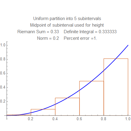
It is an example of what you see when you run the demo below.
The partition is $(0,0.2,0.4,0.6,0.8,1)$ and the evaluation points are $0.1$, $0.3$, $0.5$, $0.7$, $0.9$, so this is a sum with uniform partition and midpoints, and its norm is $0.2$. The other data given above the graph is explained later.
So the concept of Riemann Sum is complex, with several constituents and interrelationships to hold in your head all at once. Experienced math people learn concepts like this all the time. Math students have a harder time. Manipulable diagrams can help.
The fundamental theorem of the Riemann sums says that the limit of all possible Riemann sums for the function $f$ and the interval $[a,b]$, as the norm goes to zero, is exactly the value of the integral.
"All possible Riemann sums" means all possible choices of partitions of $[a,b]$ (keeping $a$ and $b$ fixed) and all possible choices of lists of evaluation points for each partition. This is a very large cloud of Riemann sums. The clouds are illustrated in these blog posts:
To do: Combine these blog posts into an article.
To do: Find a way to cut out the extra space between the demo and the following paragraph.
Note that you can use this Demo without knowing anything at all about Mathematica. There are hundreds of Demos available in the cloud that can be used in the same way; many of the best are on the Wolfram Demonstration Project.
If you can program some in Mathematica, you can take the source code for this demo and modify it, for example to use other functions, to provide functions with changeable parameters and to use partitions following dynamic rules.
A teacher in the past would draw an example of a RIemann sum on the blackboard and talk about a few features as they point at the board. Nowadays, teachers have slides with accurately drawn Riemann sums and books have pictures of them. This sort of thing gives the student a picture which (hopefully) stays in their head.
That picture is a kind of metaphor which enables you to think of the sum in terms of something that you are familiar with. The picture of a Riemann sum is not something you knew before you studied them, but your brain has remarkable abilities to absorb a picture and the relations between parts of the picture, so once you have seen it you can call it up whenever you think of Riemann sums.
I am using "metaphor" in the sense of conceptual metaphor, the way your brain partially blends two different concepts by identifying certain similarities they have. See also Metaphor in abstractmath.org.
Many other metaphors besides pictures help to understand math objects. For example, you can think of a function as position and its derivative as velocity. Position and velocity are familiar from driving or any other kind of moving. But a picture is an unusually powerful metaphor, because it calls upon your remarkable ability to understand what you see. Twenty percent of your brain is devoted exclusively to vision, and that part is connected to many other parts of the brain (balance, navigation, motor and so on).
But there are a lot of aspects of Riemann sums that cannot be demonstrated by a still picture. When the mesh gets finer, the value of the sum tends to be closer to the exact value of the integral. You can stare at the still picture and sort of visualize this. But with the demo above you can repeatedly decrease the mesh and watch the error get smaller.
An elaborate demo with lots of push buttons is something for students to play with on their own time and thereby gain a better understanding of the topic. Before manipulable diagrams the only way you could do this was produce physical models. I don't know of anyone who produced a physical model of a Riemann sum. It is possible to do so with some parameters changeable but it would be difficult and not as flexible as the demo given here.
These examples are for people who cannot manipulate the demos in this article on this computer. They should be helpful, but they are really a second-best aid.
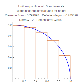
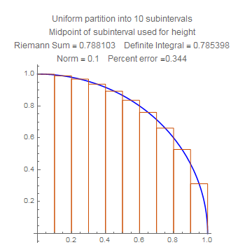
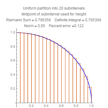
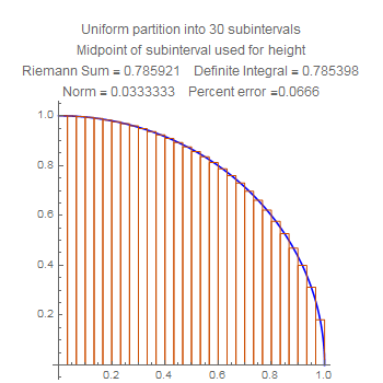
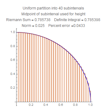
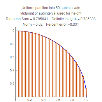
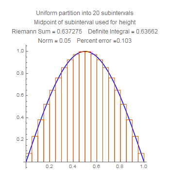
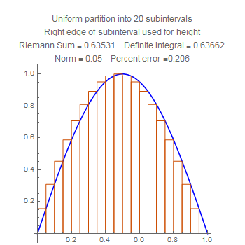
These are Riemann sums for the area of the quarter circle listed in order of the number of subintervals. Notice that the accuracy improves uniformly.
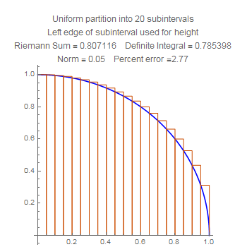
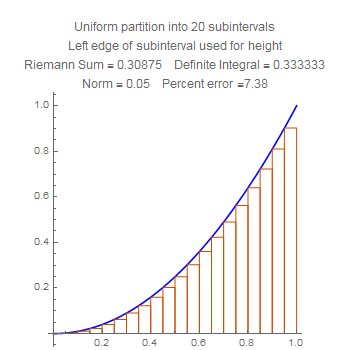
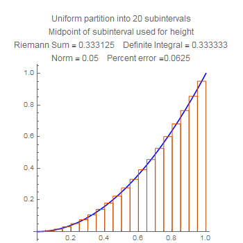
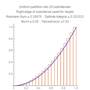
These show the quartercircle sum with twenty subdivisions, using left, middle, and right side choices of heights. Notice that the error for the midpoint is much smaller than the other two, but also that the error for the right side is worse that the error for the left side. Stare at the pictures to figure out why.

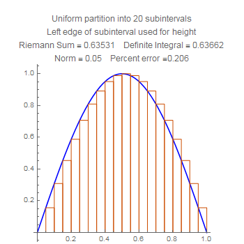
These are sums for the squaring function $x\mapsto x^2$. Notice that the difference in error between the left side heights and the right side heights are much less than for the quarter circle. Do you suppose that has to do with how big the derivative gets?
For one arch of the sine function the error is the same for the left side and the right side heights. Why?
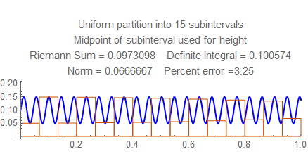
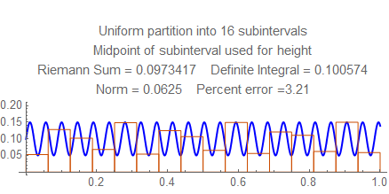
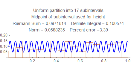
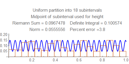
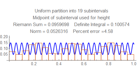
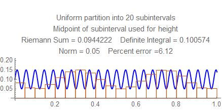
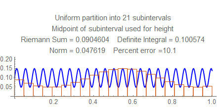
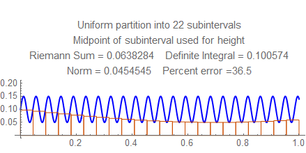
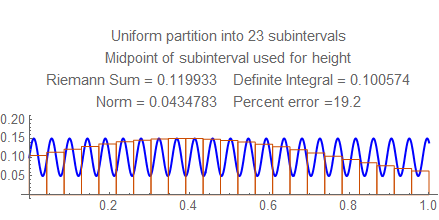
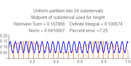
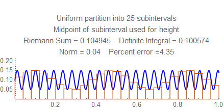
In the examples already shown, the error of the Riemann Sum generally approaches zero as the norm (width of the subintervals) approaches zero. But as all numerical analysts know, in some examples it can fluctuate wildly. If you calculate some value with just one value of the norm, you can get a wildly wrong answer. The demo below exhibits this behavior.
I once heard a talk describing how this sort of thing resulted in the collapse of an oil rig, but I no longer have a reference to it.
Check out the errors for each norm from $15$ to $25$, and notice the wild fluctuation. Then look at the errors between $50$ and $55$ (for example) and see how they steadily go down. Notice there the frequency is a little less than $22$ cycles per unit, and the rectangles in the sum resonate in some way with the waves; this won't happen at higher frequencies, when several rectangles fit into each wave.
Here are still graphs for the number of subintervals from $15$ to $25$, and below them is a table of numbers of subintervals and errors from $50$ and $55$.
Here are the errors for $50$ to $55$:
\[\begin{array}{ccccccc} \text{Number of subintervals} & 50 & 51 & 52 & 53 & 54 & 55 \\ \text{Percent error} & 0.242 & 0.23 & 0.219 & 0.209 & 0.2 & 0.191 \\ \end{array}\]The Mathematica program and the CDF player are available on Windows, Mac and Linux computers. On a Windows or Mac computer, you can run .cdf files that are embedded in html, provided that CDF player is installed on your computer and that you are viewing the html file using Firefox, Safari or Internet Explorer (not Chrome). These restrictions makes difficulties for many people; my own experience in teaching with it is that in one college I taught at briefly a few years ago, many students wanted to view my html files that contained embedded CDF files on public college computers, but most of those computers did not have CDF player installed. That included the one in the classroom I was teaching, but I got around that by bringing in my laptop.
It was those problems that led me to add some non-manipulable diagrams into this article. They do give the reader some ability to see how the different parameters in a Riemann Sum affect the accuracy of the output.
There are other possibilities that I may investigate, including movies (which can be produced by Mathematica) and using the Wolfram Cloud, which I would have to have funding to use.
This work is licensed under a Creative Commons Attribution-ShareAlike 2.5 License.